Simulation Workflow
Follow the complete Slope Optimiser workflow, from importing a section and defining properties to running simulations, reviewing results, exporting profiles, and preparing downstream models.
Follow these steps to configure a selected section in Slope Optimiser and run a simulation:
Importing Sections
Start by importing an existing DXF section or creating sections from a 3D stratigraphy model using the slicing tool.
We recommend importing sections directly if they are already defined in DXF files. This straightforward method avoids importing large 3D model files solely to create sections.
In Slope Optimiser, you have two methods available for defining cross-sections:
Importing 3D Solid/Wireframe and Making Sections
You can import a 3D solid or wireframe (File -> Import Stratigraphy -> DXF) and then use the slicing tool to create a section. For more information, refer to Creating Sections.
In the current slicing tool, click Select visible models, choose the XY, XZ, or YZ plane, and position the live clipping plane. Drag the arrow handle to move the plane. For a vertical plane, drag the circular rotation handle to rotate the plane and change its azimuth. Review the live clipped preview before clicking Slice.
Directly Importing DXF Section File
Alternatively, you can directly import a DXF section file using the pathway: File -> Import Section -> DXF.
Use Quality Input Data
Ensure your DXF model data meets general quality standards to obtain reliable simulation results. For guidance on preparing and checking data, refer to Data Preparation.
Defining Properties
Define bench, rock, general, and optional properties before running a simulation.
Define Bench Properties
Specify properties for benches if your cross-section includes them:
- Unit Weight: Weight of material per cubic metre.
- Bench Face Angle: Inclination angle of bench faces.
- Min Berm Width: Minimum width of berms between benches.
- Number of Benches: Total number of benches.
- Bench Height: Height of each bench.
Set Rock Properties
Choose between Hoek-Brown and Mohr-Coulomb models and set properties like:
- Strength characteristics.
- Friction parameters.
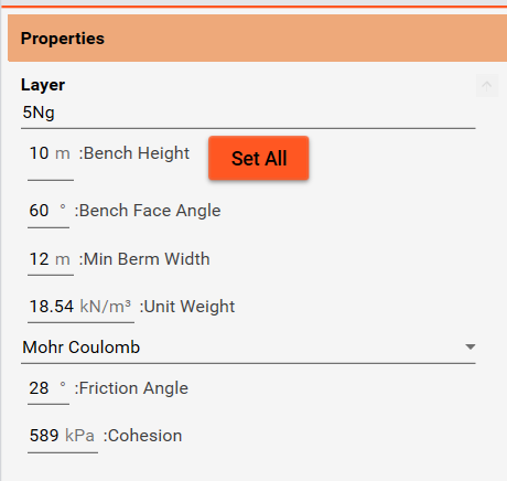
Rock properties are set separately for each section layer. Alternatively, if 3D models are used to generate sections, properties can be defined initially at the 3D model level. Sections created using the slicing tool automatically inherit these properties from their parent 3D models.
General Section Properties
Set general properties for the section:
- Slope Anchor: Choose whether the crest or toe is the fixed endpoint of the design.
- Crest anchor: Define the crest position and target slope height.
- Toe anchor: Define the toe horizontal position and elevation. The software calculates the slope height and bench-compatible height.
- Target FoS (Factor of Safety).
- Failure Direction: Select right-to-left or left-to-right slope generation.
The target slope height and bench-compatible slope height may differ. Use full benches keeps benches at their specified height and can give a slope below the target; Use target height allows a shorter crest bench to reach it. See Target and Bench-Compatible Slope Heights for examples and guidance on choosing the height option.
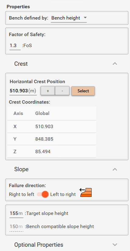
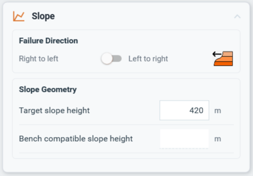
The bench, rock, and general properties described above must be provided before running a simulation. The optional properties listed below can be added if required.
Optional Properties
- Water: Water-table location and pressure method, if applicable.
- Water Pressure: Use hydrostatic pressure or apply the phreatic-line inclination correction.
- Loads: Add line loads or uniform/linear distributed loads by selecting their positions on the section topography.
- Roads: Presence and properties of roads on or near the slope.
- Tension Crack Properties: Characteristics of any tension cracks.
- Faults: Geometry and material properties of faults, if applicable. For detailed information, refer to Faults.
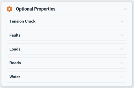
Ensure that all values accurately reflect the physical and mechanical characteristics of the materials and the specific cross-section.
For detailed guidance, refer to Properties.
Running Simulations
Configure results storage, the user profile, input checks, and the cloud simulation process.
Select the Simulation tab beside Visualiser, at the bottom of the main workspace.
Use Visualiser to inspect and prepare model geometry. Use Simulation to select a cross-section, run the analysis, and review its results. These workspaces are separate from the left-hand model navigation panel.
For help finding a control, open the SlopeOptimiser Assistant in this manual and ask, for example, “Where is the Simulation window?”
Overview
Slope Optimiser runs computationally intensive simulations in the cloud to avoid overloading local resources or affecting the performance of the user’s computer.
After the simulation problem has been defined with the required inputs, use the simulation window to run the analysis and obtain results.
Configuring the user profile
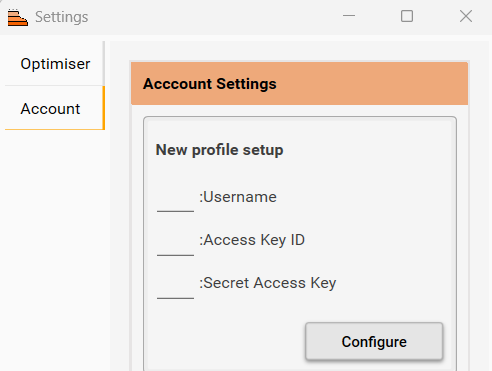
- To run simulations in the cloud, configure the user profile under Tools > Settings > Account.
After the input data is defined, simulations can be started in the simulation window. Follow these steps before starting a simulation:
- Select a section of interest. Select any section with the required properties.
- Choose the results location:
- Automatic creates a section simulation folder beside the saved project when the simulation starts.
- Custom uses a folder selected by the user.
Automatic storage requires the project to be saved as a
.cbffile first. Custom folder names may contain only letters, numbers, hyphens, and underscores.
- Make sure the user profile is configured. When running a simulation for the first time, go to
Tools -> Settings -> Account, enter the provided credentials, and click Configure. This ensures that the simulation can run in the cloud.
Common Simulation Input Checks
Before submitting a simulation, Slope Optimiser opens the Simulation Check panel when required inputs need attention. Each issue includes a description and a Fix button. Selecting Fix opens the relevant section or layer in the Properties panel and highlights the field that needs input. After correcting the values, click Check Again.
The structured check covers:
- the active crest or toe anchor and its coordinates;
- slope height where crest-anchor mode is used;
- target FoS and bench definition;
- required bench and rock properties;
- the selected strength model and its required parameters;
- cohesion and friction angle for fault layers;
- load positions, magnitudes, endpoints, and overlapping loads.
Geometry and groundwater checks that require native model processing or a user decision can still appear later while the simulation input is generated. Review those messages before choosing whether to continue.
Section Geometry Checks: Gaps and Overlaps
Before running a simulation, Slope Optimiser analyses the input section geometry and checks for common geometry inconsistencies, including gaps and overlaps.
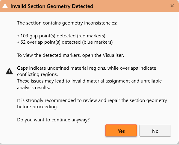
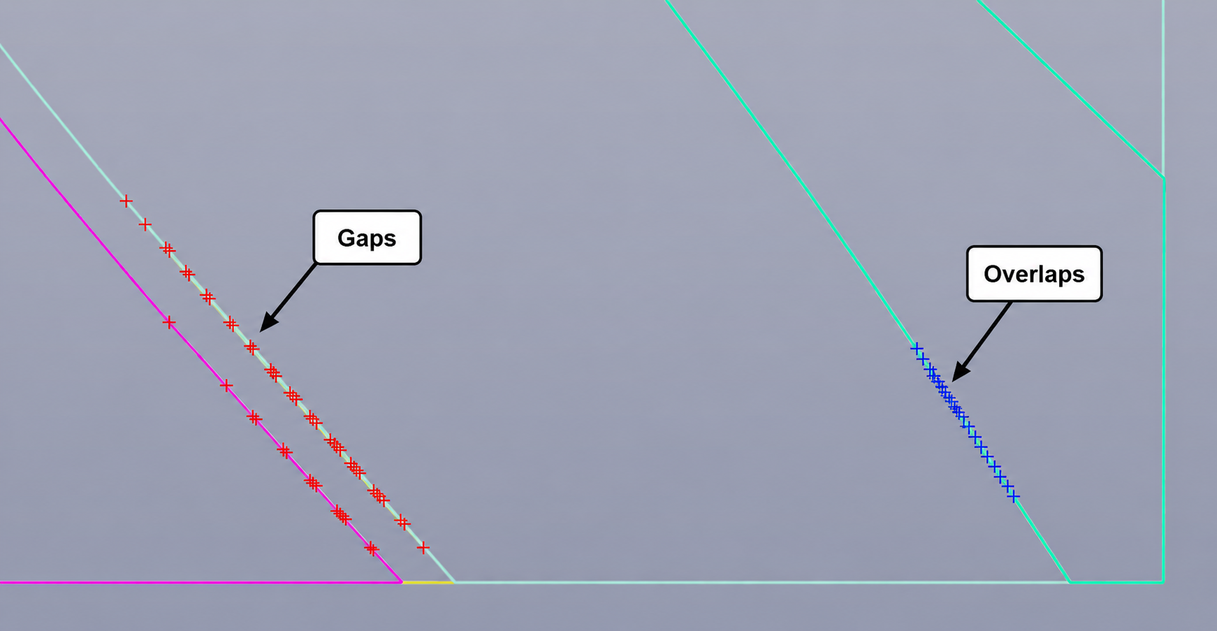
- Gaps are undefined regions between section boundaries or layer wires where material cannot be assigned clearly.
- Overlaps are conflicting regions where two or more material areas occupy the same space.
Small isolated gaps may not significantly affect the simulation result, especially if they occur away from the expected failure region. However, larger gaps or frequent gaps throughout the section can reduce the reliability of the model and may lead to less meaningful results.
Overlaps should be reviewed carefully, especially when they are easily visible in the section geometry. Overlapping regions can affect the material order assignment and may influence how the software estimates the failure mechanism.
To view detected gap and overlap markers, open the Visualiser. Gap markers are shown in red, while overlap markers are shown in blue.
Geometry Review Checklist
Before proceeding with a simulation, check the following:
- Review detected markers
- Open the Visualiser to inspect red and blue markers.
- Red markers indicate detected gap points.
- Blue markers indicate detected overlap points.
- Check the size and frequency of gaps
- Small, isolated gaps may be acceptable in some cases.
- Large or repeated gaps should be repaired before running the simulation.
- Pay particular attention to gaps near the slope face, slope toe, crest, or expected failure region.
- Check visible overlaps
- Review any overlaps that are clearly visible in the geometry.
- Correct overlaps where material boundaries cross or conflict.
- Make sure overlapping layers do not create ambiguous material regions.
- Check imported DXF quality
- Ensure section boundaries are clean and continuous.
- Remove duplicate or unnecessary lines where possible.
- Avoid very small disconnected segments or sliver regions.
- Confirm that layer wires represent the intended geological structure.
- Decide whether to continue
- If only a few minor markers are detected and they are away from the critical region, it may be reasonable to continue.
- If many markers are detected, or if the issues are near the slope profile or likely failure zone, repair the geometry first.
Recommendation:
For reliable simulation results, review and repair significant gaps and visible overlaps before proceeding. Clean section geometry improves material assignment and gives the optimiser a more reliable basis for estimating the optimal slope profile.
Slope Anchor and OSA Search Region
How should I choose the crest point?
In Crest anchor mode, the crest point defines the uppermost starting location of the slope. Its position and the target slope height directly affect how the slope geometry is generated during optimisation.
If the crest is placed too close to the outer edge of the section or terrain, the calculated slope (based on the initial maximum overall slope angle) may project outward beyond the existing ground surface. In this case, parts of the slope will extend into open space — effectively creating geometry that intersects “thin air.” This can lead to unrealistic results and may cause instability or inaccuracies in subsequent simulations.
To avoid this, position the crest point further inland, so that:
- The entire slope profile remains within the defined ground surface.
- The slope toe and face are generated against actual material, not empty space.
- The optimisation process has valid geometry to work with in all iterations.
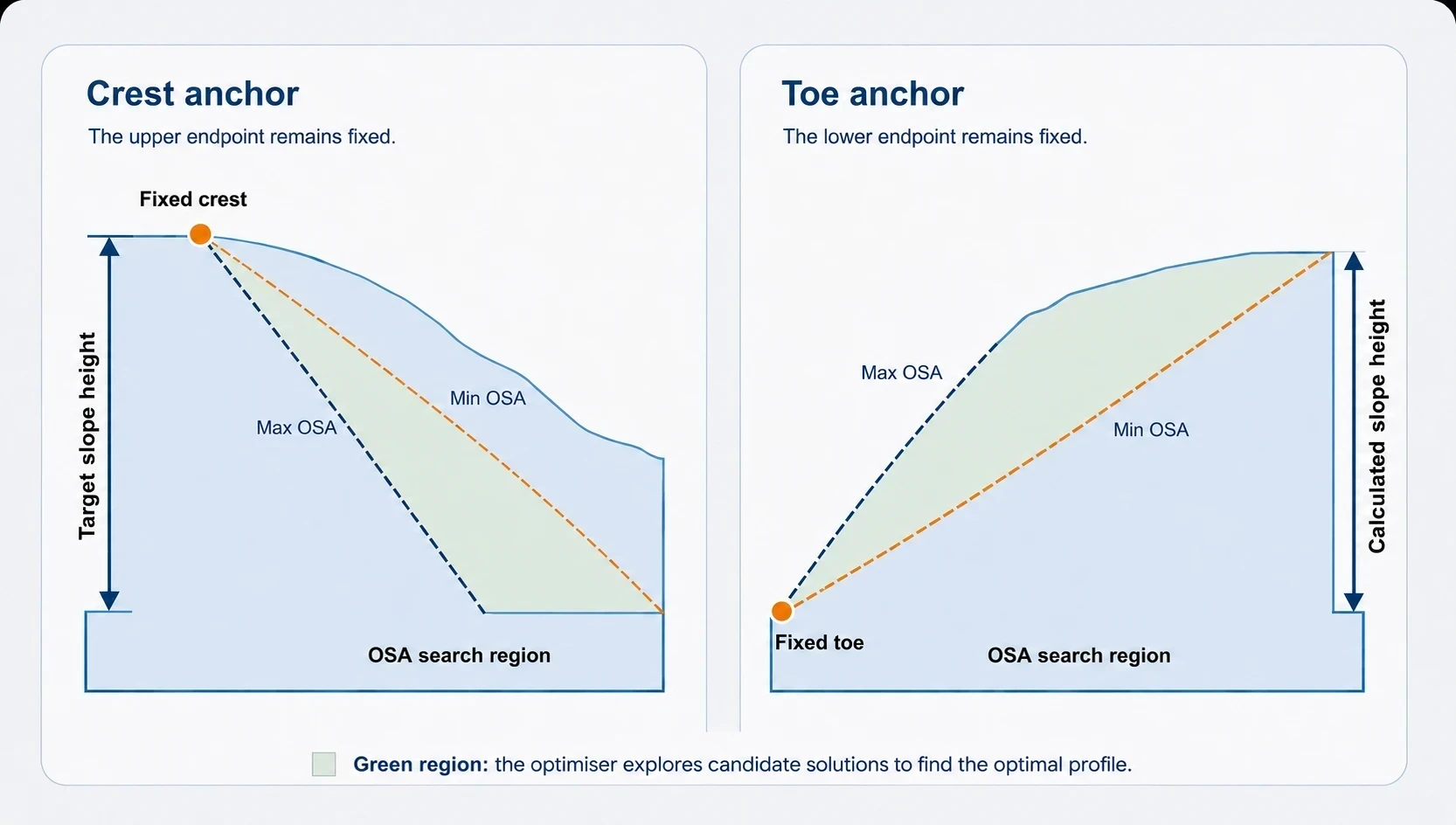
When the crest point is set correctly, the section preview shows the preliminary minimum and maximum Overall Slope Angle (OSA) limits. These are indicated by the green triangular search region. This triangle represents the area where the simulation will search for the optimal slope profile shape (see picture below).
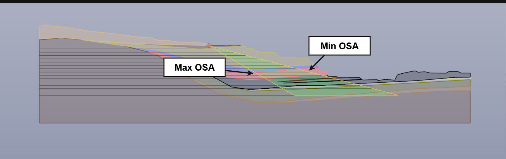
The preliminary OSA limits are calculated from the active slope anchor and the section properties. If the anchor and properties result in a very narrow difference between the minimum and maximum OSA, the simulation has only a limited search range. In this case, the optimiser will not be able to explore many possible slope profiles, which may reduce the quality or usefulness of the optimisation result.
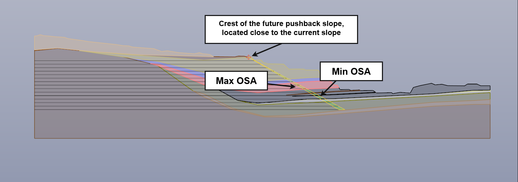
A wider, realistic OSA search range gives the optimiser more flexibility to investigate alternative slope shapes while remaining within the valid section geometry.
Practical Tips:
- Position the crest point slightly further inside the section boundary than you think is necessary.
- Check that the green triangular search region remains within the available ground/material area.
- Avoid crest point positions that create a very narrow minimum-to-maximum OSA range.
- If the green triangle is too narrow or extends outside the model, adjust the crest point or review the section properties before running the simulation.
How should I define a toe anchor?
Use Toe anchor mode when the lower endpoint of the design is known. Enter or select both the toe horizontal position and its elevation. The application calculates the slope height and bench-compatible height from the resolved toe.
The toe must remain inside the section, at or below the topography, and above the section floor. Review the estimated OSA range after every toe adjustment. Changing the toe may invalidate the existing water table; redraw or re-import it if the application removes it.
Starting Simulations
- Select the Simulation tab beside Visualiser, at the bottom of the main workspace.
- Under Cross-sections, select the desired cross-section.
- Select Automatic or Custom under Simulation results location. If using Custom, click Select folder.
- Click Start.
- Resolve any items listed under Simulation Check, then click Check Again.
- When the check passes, click Start again to begin submission.
- Continue through any geometry or groundwater warnings shown while the input is generated.
- Select your configured account if prompted. If the results folder belongs to another account, review the warning before starting a new run; choose a separate Custom folder to keep the existing results.
- Use Fetch results to download completed results or view the progress of a running simulation.
Monitoring Node Status and Output
The Simulation Output area displays a Node status summary when node information is available. Open the panel to review whether individual nodes are preparing, queued, running, complete, or failed.
- Select a node to display that node’s output in the log area.
- Click Show main output to return to the main simulation output.
- Keep Follow output selected to scroll automatically as new log lines arrive. Clear it when reviewing an earlier part of the log.
- Use the search field and Next, or press Enter, to move through matching log entries.
- Click Copy to copy the displayed output.
Creating Different Scenarios
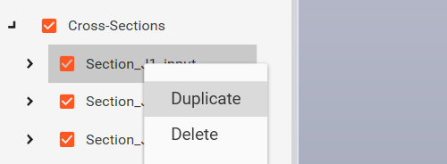
To test different design or material scenarios for the same cross-section, right-click the section in the project tree and select Duplicate. This creates an independent copy of the selected section, allowing you to modify simulation inputs without changing the original section.
Typical scenario changes may include:
- Slope geometry — adjust the slope profile, crest position, or slope height.
- Bench settings — test different bench heights, berm widths, or bench face angles.
- Material properties — compare different rock strength parameters or material models.
- Faults — evaluate the influence of different fault positions, orientations, or fault material properties.
- Water table — evaluate dry, wet, or alternative groundwater conditions.
- Loads or roads — assess line loads, distributed loads, or alternative road positions.
When running simulations for duplicated sections, make sure each scenario has either:
- A unique section name, for example:
Section_1_BaseCaseSection_1_WetConditionSection_1_LowStrength
or:
- A different results folder for each scenario.
This helps avoid conflicts between simulation outputs, logs, and exported result files. Note: When rerunning a section with corrected parameters, select Yes to overwrite the existing input data when starting the simulation.
Transferring Properties to Another Section
To reuse an existing setup on a newly imported section, open Tools > Settings > Transfer Section Properties. Select the section that should receive the properties, click Transfer Section Properties, and then choose the source section.
Review the property groups and layer mapping before confirming the transfer. Layers with the same name are matched automatically; unmatched layers can be mapped manually or excluded. Geometry-dependent data, including crest and toe coordinates, slope height, water-line points, roads, loads, simulation folders, plots, results, and result logs, is not transferred.
The receiving section must not have an active or submitted simulation. Fetch or stop that simulation before transferring properties.
Results
Slope Optimiser returns an interactive Output Plot showing the estimated optimal slope profile. In the legend, the green result line is labelled Optimal profile for mine planning. The plot toolbar can be used to:
- fit the view to the plot data using the first button on the left;
- show or hide the legend;
- choose individual visible plot items or select Show all;
- switch the embedded 2D plot between light and dark backgrounds;
- copy the plot to the clipboard;
- save the plot as a PNG or SVG image;
- open a detached plot window.
Detached plot windows are static snapshots and can be kept open side by side to compare cross-sections. From a detached window, the same cross-section can be opened in another window. Legend visibility, plot-item visibility, fit, copy, and save controls remain available.
The estimated profile coordinates and angles are also displayed in the logs, and the results folder contains the generated plots and optimal-profile data. Under Output Tools, use Create cross-section from output to add the optimised result as a new section in the project.
An example of input and output slope profile
An example of 2D output slope profile
- Note: Results in the 2D plot are always shown as if the slope is on the right side and are mirrored if the slope is on the left. When exporting the output profile to DXF or visualising it in 3D, the resulting slope profile is shown in its original position.
Exporting Output Profile to DXF
Export the optimised slope profile using global, local, or Rocscience-ready options.
Simulation results are shown in the 2D plot window and recorded in the logs. The estimated slope profile can be exported to DXF and later imported into other software.

- Navigate to the tools section in the simulation window (
Export output profile to DXF). - Select one of the export configurations:
Global- the exported profile coordinates use the original global coordinate system. This is useful when the result is visualised relative to the original section or 3D models.Local XZ- the exported profile coordinates are aligned with the XZ plane (the Y coordinate is fixed).Local XY- exported coordinates are flattened, i.e., the section is on the XY plane and is horizontal (Z coordinate is fixed). This is useful for general 2D workflows.Rocscience- exports a 2D DXF prepared for use in Rocscience software. This option automatically generates the closed external boundary required for the model, so it does not need to be drawn manually after import.
Importing Output into Rocscience RS2
Import the Rocscience-ready DXF profile with its automatically generated external boundary.
Since results from Slope Optimiser may be used in RS2 for stability analysis, this step explains how to export and import a Rocscience-ready DXF file.
Step 1: Export output profile to DXF from our software
- Export the output profile as DXF (as explained in Step 4) using the
Rocscienceexport option. The exported section is prepared as 2D geometry and includes an automatically generated closed external boundary.
Step 2: Import into RS2
- Import the DXF File: Open RS2 and import the Rocscience DXF file.
- Set Boundary Types: RS2 assigns Boundary Types based on layer names. Ensure your layer names match the expected Boundary Types in RS2. If a layer name does not match, it will be set to ‘Not Assigned’.
- Check the external boundary: Confirm that the closed outer polyline generated by Slope Optimiser is assigned as the
Externalboundary. Assign the remaining imported boundaries according to the RS2 model requirements.
By following these steps, you can successfully prepare and import a DXF file into RS2, ensuring that all elements are correctly interpreted by the software.
Exporting the Section Block Model
Export a 2D or 3D block model CSV using the optimised slope angles.
After fetching the simulation results, open Output Tools in the simulation window and click Export block model. The export opens in a separate, resizable window for the selected section.

1. Choose the export mode and block size
| Mode | Block dimensions in metres | Model requirements |
|---|---|---|
| 3D (X, Y, Z) | X, Y, Z | The section must be associated with 3D stratigraphy. |
| 2D (X, Z) | X, Z; Y is hidden | Uses the cross-section and its simulation results. No 3D stratigraphy is required. |
Smaller blocks provide more detail but produce larger CSV files. Choose dimensions appropriate for the model scale and check the total block count in the preview.
2. Set the block model origin
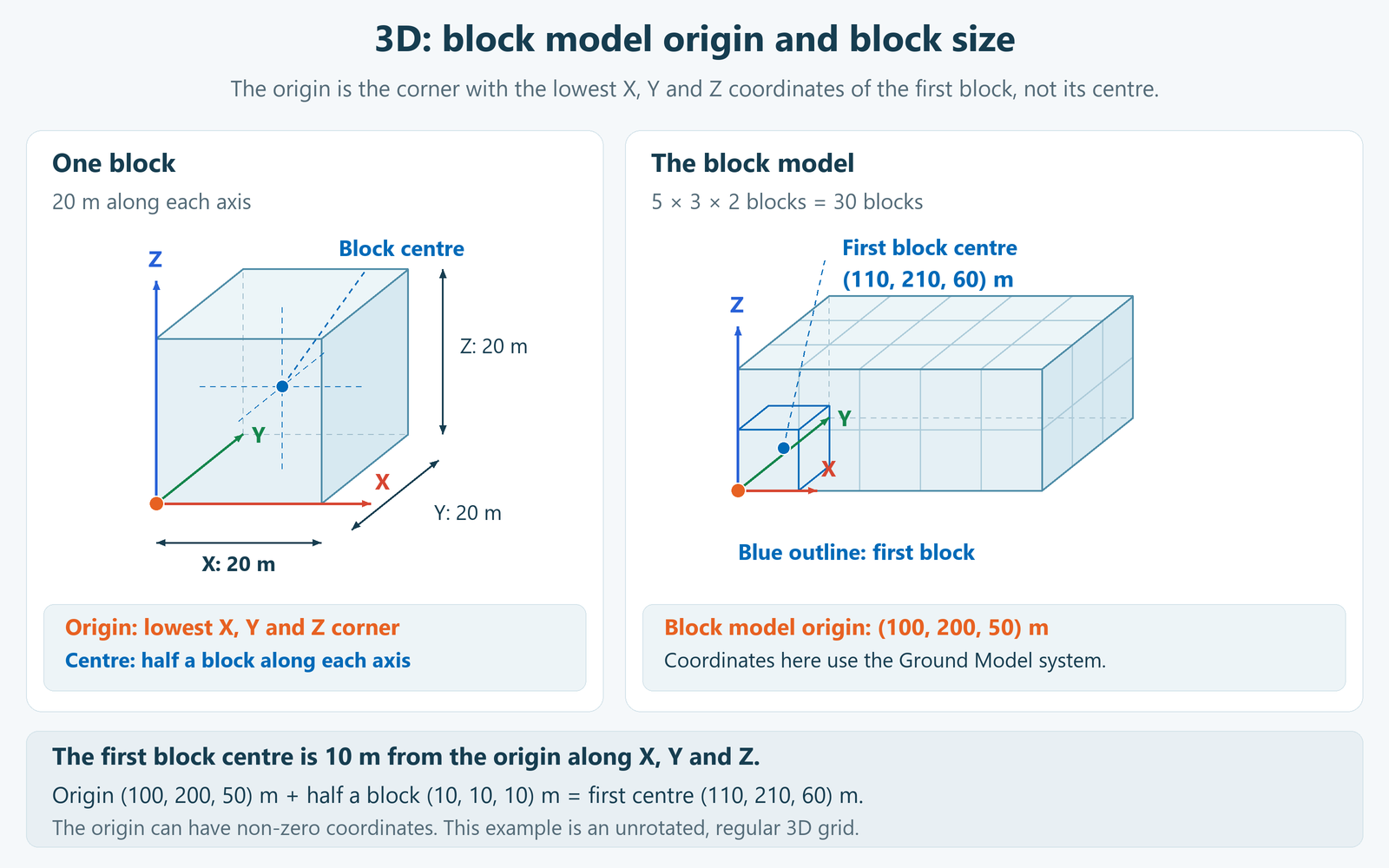
Under Block Model origin coordinates, choose Automatic to use the model bounds, or Custom position to enter the grid origin. The origin fields are read-only in Automatic mode. The origin is a block corner, not its centroid, and does not have to be zero.
A custom origin below the model bounds extends the grid; an origin inside the bounds crops its lower part. This changes the grid extent without moving the model or slope geometry. Select Automatic to restore the original lower bounds.
In the app, Explain origin and coordinates opens help for the selected export mode only. The resizable, offline window has tabs for Origin and block size and Coordinate systems.
3. Choose the exported coordinates
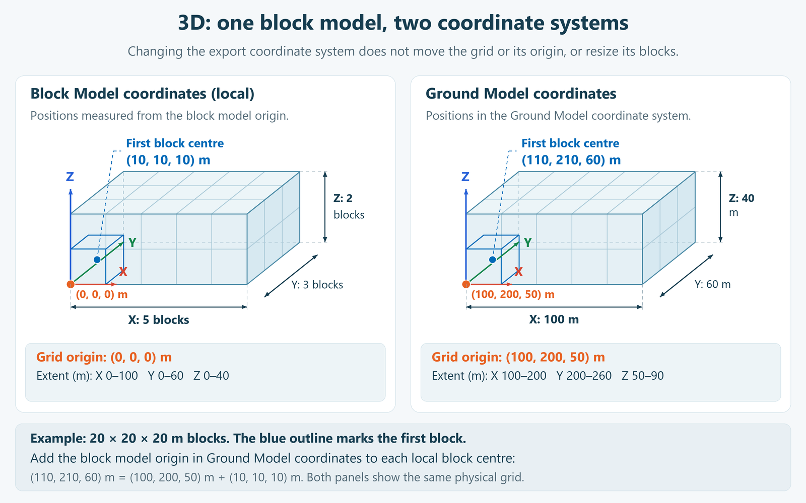
Under Export coordinate system, select the reference used for exported block centres. The First block centre readout shows the values that will be written to the CSV. Switching coordinate systems changes how positions are expressed. It does not move the grid or its origin, or change block sizes or slope angles. The same physical grid origin is expressed as zero locally and by its position in Ground Model or cross-section coordinates.
3D: origin and Ground Model coordinates
- Automatic origin: the Ground Model’s lowest X, Y and Z coordinates.
- Custom origin: enter X, Y and Z in the Ground Model coordinate system.
- Block Model coordinates (local): the grid origin is treated as (0, 0, 0).
- Ground Model coordinates: block centres retain their coordinates in the Ground Model coordinate system.
2D: origin and cross-section coordinates
- Automatic origin: the cross-section’s lowest X and Z coordinates.
- Custom origin: enter X and Z in the cross-section coordinate system.
- Block Model coordinates (local): the grid origin is treated as (0, 0).
- Cross-section coordinates: block centres retain their coordinates in the cross-section coordinate system.
For a rotated section, its X and Z coordinates are not global 3D coordinates.
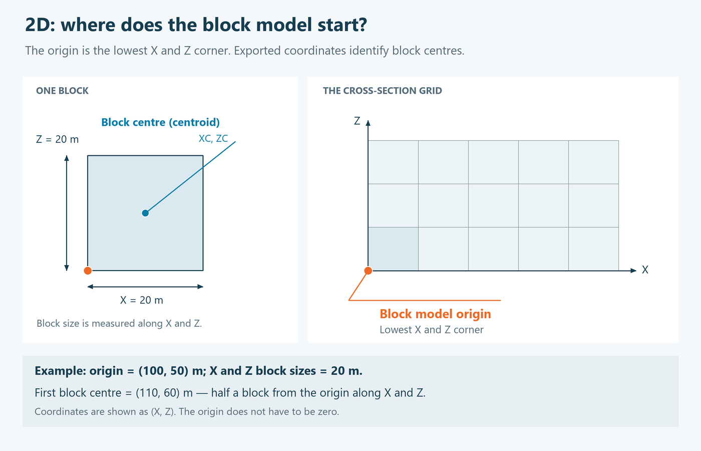
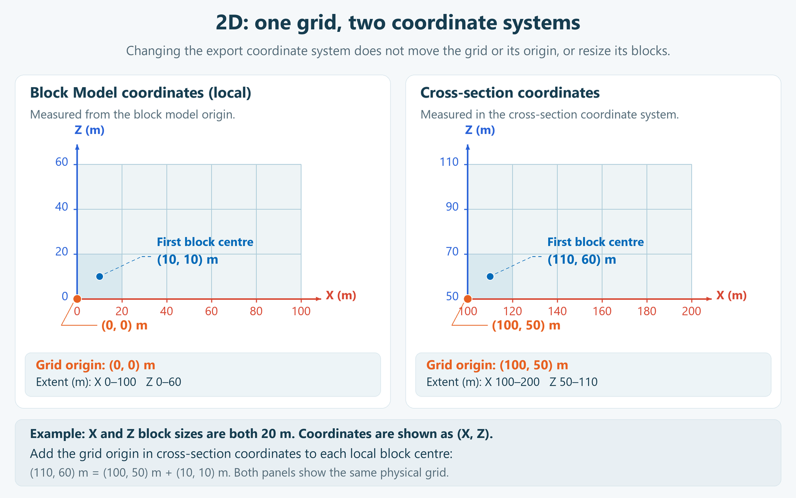
The origin is a block corner; exported coordinates are block centres. When importing or combining models, match the coordinate system, origin and block dimensions.
4. Check the preview
The preview updates when you change the dimensions, origin or coordinate option. Check the grid extent, block count and First block centre before exporting.
- Colours show slope angles in degrees; grey blocks have no angle and export with a blank
slope_anglevalue. - In 3D, drag to rotate and scroll to zoom. Axis colours are X red, Y green and Z blue.
- In 2D, pan and zoom to inspect the grid. Use Fit view to restore the full view in either mode.
The grid covers a rectangular area or volume; it is not clipped to rock boundaries or the excavation shape. Fine grid lines may be hidden at larger scales.
5. Export the CSV
Click Export CSV, choose a file name and save location, and save the file. If export is unavailable, follow the explanation shown in the window and check the results, model requirements and input values. Grids larger than 10 million blocks require larger block dimensions or a smaller extent.
The CSV contains block centre coordinates, block dimensions and slope_angle in degrees:
- 3D:
X, Y, Z, dX, dY, dZ, slope_angle - 2D:
X, Z, dX, dZ, slope_angle
For a 3D Datamine workflow, continue with Import Block Model into Datamine.
Import Block Model into Datamine
Import the block model CSV exported from OptimalSlope into Datamine, assign the correct block model fields, and combine the slope-angle output with the original block model.
This step explains how to import an OptimalSlope block model export into Datamine. The workflow is split into two parts:
- Import the main block geometry and save it with a clear base-model name, for example
Block_Model_XYZ. - Import the OptimalSlope slope-angle output, save it with a clear slope-model name, and combine it with the original model using
ADDMOD.
The CSV should contain the block dimensions, block centre coordinates, and any extra attributes such as density, grade, rock type, lithology, or slope angle.
1. Import an external block model file
In Datamine, select the option to import an External file.
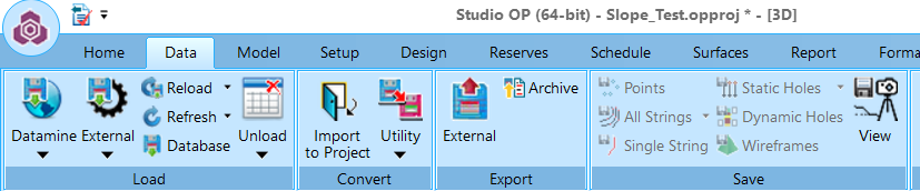
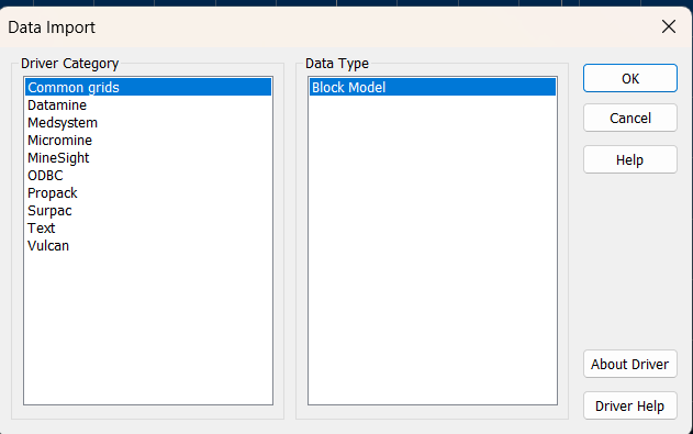
In the Data Import window:
- Select Text as the driver category.
- Select Block Model as the data type.
- Click OK.
2. Specify model parameters
Specify the block model parameters:
- Model Origin — enter the X, Y, and Z origin values.
- Block Size — enter the X, Y, and Z block dimensions.
- Number of Blocks — enter the number of blocks in X, Y, and Z.
Use the same dimensions and coordinate frame as the export. With Ground Model coordinates, use the export’s Ground Model origin. With Block Model coordinates (local), the grid origin is zero on each axis. The First block centre is not the model origin.
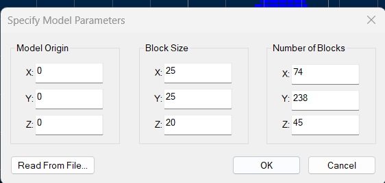
Click OK to start the import wizard.
3. Configure the text wizard
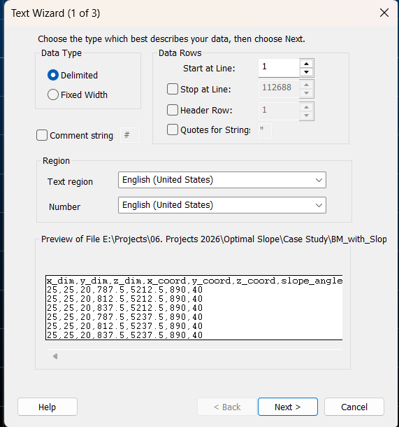
In Text Wizard 1 of 3:
- Set Data Type to Delimited.
- Set Header Row to
1. - Check that the preview shows the expected CSV columns.
- Click Next.
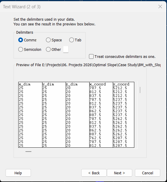
In Text Wizard 2 of 3:
- Select Comma as the delimiter.
- Confirm that each CSV field is separated into its own column.
- Click Next.
4. Assign Datamine field types
In Text Wizard 3 of 3, assign the field type for each imported column.
Use the following mapping for the main block model:
| CSV field | Datamine field type | Data type | Purpose |
|---|---|---|---|
X_dim | XINC | Numeric | Block size in the X direction. |
Y_dim | YINC | Numeric | Block size in the Y direction. |
Z_dim | ZINC | Numeric | Block size in the Z direction. |
X_coord | X | Numeric | Block centre X coordinate. |
Y_coord | Y | Numeric | Block centre Y coordinate. |
Z_coord | Z | Numeric | Block centre Z coordinate. |
Additional fields may include:
- Density
- Grades
- Rock Type
- Lithology
- Other project-specific attributes
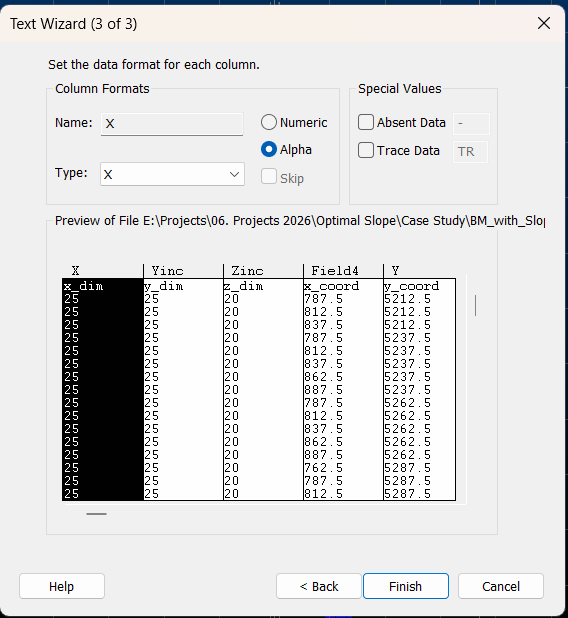
Click Finish. The block model should be displayed in Datamine.
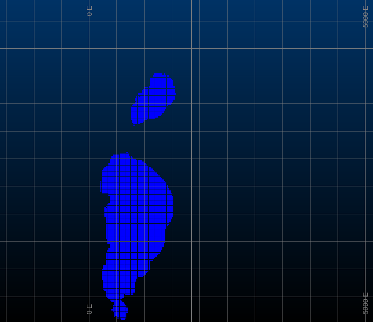
Save the imported Datamine block model with a clear name. In this tutorial, the suggested example name is:
Block_Model_XYZ
You may use another valid Datamine file name, as long as you can clearly identify it later as the base block model.
5. Import the OptimalSlope slope-angle model
Repeat the import workflow for the model that contains the OptimalSlope slope-angle output.
For the 3D OptimalSlope CSV, map X, Y and Z to Datamine coordinate fields X, Y and Z; map dX, dY and dZ to XINC, YINC and ZINC. These column names differ from the example base-model fields above. Check that both models use the same coordinate system, origin and block dimensions before combining them.
The slope-angle field should be imported as:
| Field | Datamine field type | Data type |
|---|---|---|
slope_angle | Attribute | Numeric |
Save this imported model with a clear name. In this tutorial, the suggested example name is:
Block_Model_Slope
You may use another valid Datamine file name, as long as you can clearly identify it later as the slope-angle model.
6. Combine the two block models
Run the Datamine function:
ADDMOD
Use ADDMOD to add the slope-angle model to the base block model, then save the output as a new Datamine block model file. In this example, Block_Model_Slope is added to Block_Model_XYZ, but the exact file names can be changed.
The names Block_Model_XYZ and Block_Model_Slope are examples only. Datamine does not require these exact names. Use consistent, recognisable names so the correct base model and slope-angle model are selected in ADDMOD.
The final output should combine:
- the original block model fields;
- the OptimalSlope slope-angle data;
- any other attributes imported from the CSV file.
After combining the models, check that all relevant blocks have a slope-angle value assigned.
Related pages
Use these pages to start faster, understand common terms, or troubleshoot issues found during the workflow.
Run through the shortest route from prepared data to simulation results.
Review common problems with geometry, OSA search region, simulation setup, and exports.
Review key OptimalSlope, slope design, simulation, and export terms.
results matching ""
No results matching ""
Try a shorter phrase or one of the suggested searches above.