Properties
Reference guide for slope anchors, bench and rock inputs, loads, faults, roads, and groundwater settings used to define simulations.
Defining Bench Height
Bench height can be fixed for a section or inherited from a parent 3D rock model during slicing.
At this stage, a fixed bench height is used for each rock or section layer.
When working with 3D rock models, if a bench height is defined, it is automatically inherited by the section from its parent shape during the slicing operation. This ensures consistency between the 3D model and the generated section geometry. If required, the section’s bench height can be edited later.
By default, bench height is set by specifying a bench height for either:
- a section, or
- a 3D rock model (stratigraphy).
Alternatively, in the section properties, the bench height can be estimated by specifying:
- the number of benches, and
- the slope height.
The software will calculate the corresponding bench height automatically.
For example, if slope height = 120 m and number of benches = 12, then bench height = 10 m.
Bench-compatible slope height is the greatest height that accommodates full benches at their specified heights without exceeding the target slope height.
For example, slope height = 385 m and bench height = 10 m gives a bench-compatible slope height of 380 m. Adding another full bench would exceed the defined slope height.
See Target and Bench-Compatible Slope Heights for the difference between retaining full-height benches and using a shorter crest bench to reach the target.
Bench Properties
Bench properties describe the basic geometry and unit weight used for bench generation.
| Name | Measurement type | Info |
|---|---|---|
| Unit Weight | kN/m³ | Unit weight in kN/m³. |
| Bench Face Angle | Degrees | Bench face inclination. |
| Min Berm Width | m | Minimum berm width. |
| Number of benches | - | Number of benches, set only if Bench defined by = No. of benches. |
| Bench Height | m | The height of each bench. |
Rock Properties
Rock strength properties are set according to the selected strength model.
Hoek-Brown or Mohr-Coulomb properties are set depending on the strength model of the material type.
| Name | Measurement type | Info |
|---|---|---|
| σ_ci | MPa | Unconfined compressive strength of the intact rock. |
| Geological Strength Index | - | Geological Strength Index for the rock mass. |
| Intact rock m_i value | - | Value controlling the Hoek-Brown curvature. |
| σ3_max | MPa | Minor principal stress averaged along the likely slope failure surface. If unavailable, set to -1. |
| Disturbance Factor | - | Factor accounting for rock mass strength reduction due to stress relaxation and blasting. |
| Name | Measurement type | Info |
|---|---|---|
| Friction Angle | Degrees | Angle of shearing resistance, also known as internal friction, of the rock mass. |
| Cohesion | kPa | Cohesion of the rock mass. |
Bench and rock properties can be set for individual 3D stratigraphic models. If sections are generated using the slicing tool, they automatically inherit these properties. If sections are imported directly, properties can be set manually for each layer in a particular section.
General Section Properties
General section properties define the fixed slope endpoint, slope geometry, target factor of safety, loads, and road inputs.
| Name | Measurement type | Info |
|---|---|---|
| Slope Anchor | - | Selects the fixed endpoint used to define the slope: Crest or Toe. |
| Crest Position | m | Local horizontal crest coordinate. Available when Crest is the active slope anchor. |
| Toe Position | m | Local horizontal toe coordinate. Available when Toe is the active slope anchor. |
| Toe Elevation | m | Vertical toe coordinate. It can be entered or selected in the visualiser after the toe position is defined. |
| Target Slope Height | m | Target slope height in crest-anchor mode. In toe-anchor mode, slope height is calculated from the selected toe and section geometry. |
| Bench-Compatible Slope Height | m | Calculated height of the full-bench arrangement that fits within the target slope height. It may be lower than the target. |
| Target FoS | - | Target factor of safety. |
| Failure Direction | - | Defines whether failure and slope generation proceed from right to left or left to right. |
| Road width | m | Width of a road. |
| Road Vertical Position (Z) | m | Road Z position coordinate. |
Target and Bench-Compatible Slope Heights
The two heights describe different aspects of the slope geometry:
- Target slope height is the requested overall vertical height, not the height of an individual bench. In Crest anchor mode, enter it in the Slope Geometry panel.
- Bench-compatible slope height is the height that can be formed using full benches at their specified heights without exceeding the target. It matches the target when the benches fit exactly; otherwise, it is lower because another full bench would exceed the target.
For example, with a 330 m target and a uniform bench height:
| Bench height | Height option | Bench arrangement | Resulting slope height |
|---|---|---|---|
| 15 m | Use full benches | 22 full benches × 15 m | 330 m — exact fit |
| 20 m | Use full benches | 16 full benches × 20 m | 320 m — below the target |
| 20 m | Use target height | 16 full benches × 20 m + one 10 m crest bench | 330 m — reaches the target |
With 20 m benches, a seventeenth full bench would give 340 m, exceeding the 330 m target. Use target height reaches the target slope height by shortening the top (crest) bench if needed. All other benches keep their specified height.
Select Use full benches when every bench must keep its specified height. Select Use target height when the requested overall height is needed and a shorter crest bench is acceptable.
The panel displays the button for changing the current height option. After using the target height, Use full benches returns to the full-bench arrangement. Target-height conversion applies in Crest anchor mode with Bench definition set to Bench height and the same positive bench height assigned to every rock layer.
Hover over either height field to read its explanation. The tooltip appears beside the field and closes when the pointer moves onto either height-conversion button.
In Toe anchor mode, define the toe position and elevation instead of entering a crest-mode target height. The software calculates the slope height and bench-compatible height from the toe and section geometry.
The Slope Anchor is the fixed endpoint used to generate the candidate slope geometry.
- Select Crest when the upper endpoint is fixed by topography, a pit limit, or the planned crest alignment. Define the crest position and target slope height.
- Select Toe when the lower endpoint is fixed by the pit floor, haul road, excavation boundary, or another design constraint. Define the toe horizontal position and elevation; the slope height and bench-compatible height are calculated automatically.
- The property panel displays the resolved global coordinates and the estimated minimum and maximum OSA for the active anchor.
Choose the anchor based on which endpoint must remain fixed, then set Failure Direction separately to match the slope orientation.
The animation below shows how changing the anchor keeps either the crest or toe fixed and updates the related slope values.
The toe must lie inside the section, at or below the topography, and above the section floor. Toe elevations are resolved to the whole-unit elevation used by the solver. If a new value is invalid, review the message in the interface and adjust the toe position or elevation.
Water-table update required: Changing the active anchor or toe geometry can invalidate an existing water table. If the application removes the water table, redraw or re-import it after the slope geometry is finalised.
The crest point defines the uppermost starting location of the slope in the model. Its position directly affects how the slope geometry is generated during optimisation.
If the crest is placed too close to the outer edge of the section or terrain, the calculated slope, based on the initial maximum overall slope angle, may project outward beyond the existing ground surface. In this case, parts of the slope will extend into open space, effectively creating geometry that intersects “thin air.” This can lead to unrealistic results and may cause instability or inaccuracies in subsequent simulations.
To avoid this, position the crest point further inland, so that:
- the entire slope profile remains within the defined ground surface,
- the slope toe and face are generated against actual material, not empty space,
- the optimisation process has valid geometry to work with in all iterations.
When the crest point is set correctly, the section preview shows the preliminary minimum and maximum Overall Slope Angle (OSA) limits. These are indicated by the green triangular search region. This triangle represents the area where the simulation will search for the optimal slope profile shape.
The preliminary OSA limits are calculated from the selected crest point and the section properties. If the crest point and properties result in a very narrow difference between the minimum and maximum OSA, the simulation has only a limited search range. In this case, the optimiser will not be able to explore many possible slope profiles, which may reduce the quality or usefulness of the optimisation result.
A wider, realistic OSA search range gives the optimiser more flexibility to investigate alternative slope shapes while remaining within the valid section geometry.
- Position the crest point slightly further inside the section boundary than you think is necessary.
- Check that the green triangular search region remains within the available ground/material area.
- Avoid crest point positions that create a very narrow minimum-to-maximum OSA range.
- If the green triangle is too narrow or extends outside the model, adjust the crest point or review the section properties before running the simulation.
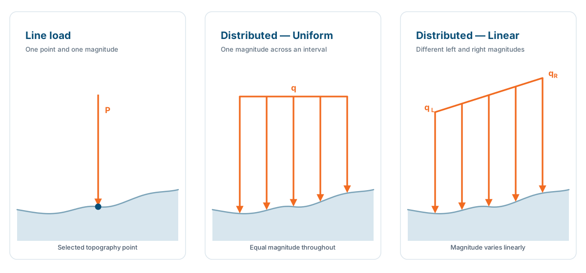
Loads are defined under Optional Properties > Loads and placed directly on the section topography.
| Load type | Selection | Magnitude |
|---|---|---|
| Line | Select one point on the topography. | Enter one magnitude greater than zero. |
| Distributed — Uniform | Select the left and right endpoints of the loaded interval. | Enter one magnitude greater than zero. |
| Distributed — Linear | Select the left and right endpoints of the loaded interval. | Enter left and right magnitudes. Both must be non-negative and at least one must be greater than zero. |
To add a load:
- Choose Line or Distributed. For a distributed load, also choose Uniform or Linear.
- Enter the required magnitude value or values.
- Click Select and choose the point or interval on the section topography. The pointer snaps to valid topography positions.
- Review the new entry in the load table.
Loads may not overlap. If the selected location overlaps another load, the existing load is highlighted and the new load is not accepted. Select a different position or delete the conflicting entry. Use Cancel to leave selection mode and Delete to remove the selected load.
The animation below demonstrates a line load, a distributed linear load with different endpoint magnitudes, and a distributed uniform load with one fixed magnitude. It also shows the warning displayed when a new load overlaps an existing load.
Roads remain separate optional inputs and are defined using their width and vertical position.
Transfer Section Properties
Copy reusable settings and mapped layer properties from an existing section to another section in the same project.
Open Tools > Settings > Transfer Section Properties, select the newly imported or receiving cross-section, and click Transfer Section Properties. In the transfer window, select the source section and choose what to copy:
The animation below shows properties being transferred from an existing section to a receiving section with different geometry. The receiving section gains the selected reusable properties while retaining its own geometry.
- Section settings — target FoS, bench and strength-model definitions, water-pressure option, and maximum fault segment length.
- Entity types — rock material, fault/joint, or piezometric-line classification.
- Layer properties — defined material, strength, and bench-property values.
The layer table automatically includes unique exact-name matches. Review every mapping, manually select a source layer where required, and clear Include for layers that should remain unchanged. A source layer can be mapped only once. Blank numerical fields in the source do not overwrite defined values in the receiving section.
Not transferred: Crest and toe coordinates, slope height, water-line points, roads, loads, simulation folders, plot data, simulation results, and result logs remain tied to their original geometry or simulation. The receiving section keeps its own geometry-dependent data. If it already has results, they are retained but marked as out of date after transferred properties change the setup.
Properties cannot be transferred while the receiving section has an active or submitted simulation. Use Fetch results or stop the simulation first.
Faults
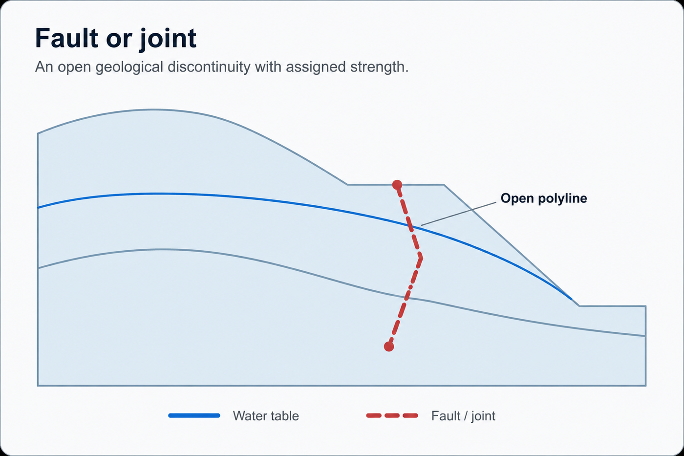
Faults represent discontinuities or fractures that can influence rock mass behaviour, stability, and stress distribution.
Faults represent discontinuities or fractures within the geological model that can influence rock mass behaviour, stability, and stress distribution.
In the Slope Optimiser, faults are defined as open polylines and can be added to a section in two different ways.
Assign faults in an imported section
- Import the DXF file as a regular section.
- In the Explorer menu, locate and select the layer containing the fault geometry.
- Tick This entity is a fault/joint (open polyline).
- Assign the fault properties shown below.
Import faults as a separate DXF
- In the Explorer menu, select the target section.
- In the Properties panel, open Optional Properties > Faults.
- Click Add to import the fault DXF file.
- Assign the fault properties in the fault layer properties.
The Maximum Fault Segment Length parameter is defined under Optional Properties > Faults.
| Name | Measurement type | Description |
|---|---|---|
| Maximum Fault Segment Length | m | Controls how imported fault polylines are segmented for analysis. Higher values create fewer segments and allow faster computation, while lower values create more segments and provide a more detailed representation of the fault geometry. The default value is 20 m. |
The following properties are assigned to the imported fault or joint polyline layer.
| Name | Measurement type | Description |
|---|---|---|
| Friction Angle | Degrees | The angle of shearing resistance, also known as internal friction, of the fault material. |
| Cohesion | kPa | The cohesive strength of the fault material, measured in kilopascals. |
The Maximum fault segment length parameter controls how imported fault polylines are divided into smaller segments for analysis.
Creates fewer fault segments, which can reduce computation time and make the simulation faster. The fault geometry may be represented in a simplified form.
Creates more fault segments, providing a more detailed fault representation. This increases computational effort and may make the simulation slower.
Use a segment length that is appropriate for the scale and complexity of the fault geometry. For simple or long faults, the default value of 20 m is usually a good starting point. For highly curved, short, or complex fault geometries, a smaller value may be useful.
Faults should be defined where they are expected to have a meaningful influence on the slope, such as where a fault crosses the slope face, slope toe, or potential failure region.
When defining faults, make sure that:
- the fault geometry is correctly positioned relative to the section,
- the fault intersects the relevant part of the slope model if it is expected to influence the result,
- fault material properties are representative of the expected geological conditions,
- the fault is included only where it is geologically justified.
When testing fault sensitivity, duplicate the section and create separate scenarios with different fault positions, orientations, or material properties.
Water Table
The water table, also referred to as the piezometric line, can be defined for a selected cross-section.
The water table, also referred to as the piezometric line, can be defined for a selected cross-section under:
Cross-section > Optional Properties > Water
Select the pressure method that matches the analysis assumptions:
- Inclination-corrected accounts for the gradient of the phreatic line:
u = γw hw cos² α. - Hydrostatic applies no inclination correction:
u = γw hw.
Here, γw is the unit weight of water, hw is the water head, and α is the inclination of the water-table segment. Confirm the selected method before running the simulation, particularly when the piezometric line is steep.
Hydraulic conductivity is not currently available as an editable interface input.
The water table is displayed as a blue polyline in the section visualiser.
| Column | Description |
|---|---|
| Index | Point index, starting from 1 at the slope toe and continuing to N at the last boundary point. |
| Vertical Position (Z) | Z coordinate of the corresponding bench line where the point is located. This value is fixed to the bench Z position. |
| X | Horizontal coordinate of the water table point. This value is editable. |
To define the water table:
- Click Draw.
- In the visualiser, select the slope toe on the lowest bench line to add the first water table point.
- Move upwards through the section, selecting one water table point on each required bench line.
- To close the piezometric line, hover over the section boundary on the left or right side, depending on the section orientation. When a valid boundary point is detected, a red circle is displayed around it. Select the highlighted point to add the final boundary point.
- Press Enter to confirm, or press Esc to cancel.
If a water table was previously imported from a DXF file, the application asks which water table to use for the simulation. Select Yes to use the manually drawn points instead, or No to keep the imported water table.
The animation below shows the complete drawing workflow, from selecting the first point at the toe to confirming the final point at the section boundary.
- Define the water table from the slope toe upwards, beginning on the lowest bench line.
- Only one water table point is allowed per bench.
- The water table should be defined so that it follows the expected groundwater conditions for the selected cross-section.
Related help
Use these pages for the recommended first workflow, common issue checks, and terminology.
- Quick Start — shortest route through the first simulation workflow.
- Help and Solutions — common geometry, OSA search region, simulation, and export checks.
- Glossary — definitions of common OptimalSlope terms.
results matching ""
No results matching ""
Try a shorter phrase or one of the suggested searches above.